TLDR; This blog post uses APIs about German highway data to display those in Kibana Vector layers in Kibana Maps using the Elastic Stack. Also, you will learn a little bit of the Crystal programming language in order to import data from JSON APIs.

The API

Everything started with this gist, where Lilith documented the API endpoints.

The API evolves around highways. There is one endpoint, that returns all the available highways and then there are several endpoints for each highway listing

• Electric Charging Stations
• Roadworks
• Closures
• Webcams
• Warnings
• Parking

You can also get more details for each of the entries returned, but in our case this was not needed.

All of the documents have a similar structure, so let’s take a look at the response of electric charging stations at the A29 - a highway I got to know well, when I studied… like almost two decades ago 😮 (that also explains the grey hair, different story though).

So, you can open the following URL to check for all charging stations on that highway:

https://verkehr.autobahn.de/o/autobahn/A29/services/electric_charging_station

One of the four elements in the returned array looks like this:

{
  "electric_charging_station": [
    {
      "extent": "8.220136,53.044915,8.220136,53.044915",
      "identifier": "RUxFQ1RSSUNfQ0hBUkdJTkdfU1RBVElPTl9fMTIyMzY=",
      "routeRecommendation": [],
      "coordinate": {
        "lat": "53.044915",
        "long": "8.220136"
      },
      "footer": [],
      "icon": "charging_plug_strong",
      "isBlocked": "false",
      "description": [
        "A29 | Cloppenburg | Raststätte Huntetal West (1)",
        "26203 Wardenburg",
        "",
        "Ladepunkt 1:",
        "AC Kupplung Typ 2",
        "43 kW",
        "",
        "Ladepunkt 2:",
        "DC Kupplung Combo, DC CHAdeMO",
        "50 kW"
      ],
      "title": "A29 | Cloppenburg | Raststätte Huntetal West (1)",
      "point": "8.220136,53.044915",
      "display_type": "STRONG_ELECTRIC_CHARGING_STATION",
      "lorryParkingFeatureIcons": [],
      "future": false,
      "subtitle": "Schnellladeeinrichtung"
    },
    {
      ...
    }
  ]
}

There are a few interesting fields in the response:

• identifier seems to be a unique identifier
• coordinate lists the latitude and longitude. Unfortunately someone decided to ignore RFC7946 and just pick an arbitrary name for the longitude, so that this needs modification for proper indexing into an Elasticsearch geo point.
• title, subtitle and description make a good candidate for a complete textual representation
• display_type contains some more information what kind of charging station this is. Can be one of ELECTRIC_CHARGING_STATION or the above STRONG_ELECTRIC_CHARGING_STATION. This field is also filled for all other data like closures or parking.

Retrieving the data and indexing into Elasticsearch

I wrote a small crystal program to index the data into Elasticsearch. If you don’t have crystal installed yet, check out the installation instructions to follow along. I’ll explain the program step by step - the code without comments is not even a hundred lines to retrieve all the data and index it into Elasticsearch.

The full crystal program is available in this gist, so you don’t have to copy & paste it from here. It’s not even a hundred lines of code.

First we parse the optional command line options

directory = "./data"
elasticsearch_endpoint = URI.parse "http://localhost:9200"

OptionParser.parse do |parser|
  parser.banner = "Usage: autobahn-api-to-es [arguments]"
  parser.on("-d", "--directory", "Directory to dump the JSON into, default [#{directory}]") { |d| directory = d }
  parser.on("-e", "--elasticsearch", "Elasticsearch endpoint, must be an URI, may contain a user:password like https://user:pass@example.org, default [#{elasticsearch_endpoint}]") { |e| elasticsearch_endpoint = URI.parse e }
  parser.on("-h", "--help", "Show this help") do
    puts parser
    exit
  end
  parser.invalid_option do |flag|
    STDERR.puts "ERROR: #{flag} is not a valid option."
    STDERR.puts parser
    exit(1)
  end
end

One small trick to not need to parse additional basic auth information is to be able to hide it in the URI, as shown in the help. So there is no need to modify this tool if you are indexing into an Elastic Cloud cluster - unless you are using API keys.

Also note, that there are two default settings for the options. First the default Elasticsearch endpoint being localhost and second the data directory. The basic idea of that directory is store the downloaded JSON, so that subsequent calls don’t need to download this again. This is merely to shorten development cycles, so if you do not want to use this feature, you can delete the contents of that data directory right after running this script or specify an argument with a temporary directory like --data $(mktemp -d).

Next it is time for some setup:

directory = directory.chomp "/"
Dir.mkdir_p directory

client = HTTP::Client.new URI.parse "https://verkehr.autobahn.de/"
es_client = HTTP::Client.new elasticsearch_endpoint
es_headers = HTTP::Headers{"Content-Type" => "application/x-ndjson"}

NOW = Time::Format.new("%FT%T.%L%z").format(
  Time.local(Time::Location.load("Europe/Berlin")))

This creates the data directory and initializes the two HTTP clients being used - one for the autobahn API and one for the Elasticsearch node.

Two helper methods are needed, first read_from_file_or_retrieve:

def read_from_file_or_retrieve(endpoint : String, directory : String, client : HTTP::Client)
  endpoint_as_file = endpoint.gsub "/", "_"
  path = "#{directory}/#{endpoint_as_file}.json"
  if !File.exists?(path)
    response = client.get endpoint
    File.write path, response.body
    JSON.parse response.body
  else
    JSON.parse File.read path
  end
end

This uses the data directory to check if there is a file downloaded from an earlier execution and uses this as JSON input if it exists. The second method processes a JSON response from one of the endpoints and parses the items in the response array:

def process_json_documents (key : String, type : String, bulk : String::Builder, json : JSON::Any)
  json[key].as_a.each do |obj|
    obj.as_h["@timestamp"] = JSON::Any.new NOW
    # set a type to filter out in queries
    obj.as_h["type"] = JSON::Any.new type
    bulk << %Q({ "index" : { "_id": "#{obj["identifier"].as_s}" }}\n)
    # move 'long' longitude to 'lon' to create elasticsearch geo_point properly
    obj["coordinate"].as_h["lon"] = obj["coordinate"]["long"]
    obj["coordinate"].as_h.delete "long"
    bulk << obj.to_json
    bulk << "\n"
  end
end

As all the data of all the endpoints that are being fetched are put into the same index, we need an additional type to identify documents. This will be used as a filter later. On top of that each obj from the JSON array is basically converted into the bulk format that Elasticsearch understands - one header line setting the id, plus one metadata line containing the document.

As already mentioned above, this requires a conversion from the geo point name for the longitude, from long to lon which happens here as well.

The passed string builder will contain the newly added documents.

Before we start retrieving data, all the data is deleted on the Elasticsearch side plus ensuring that the coordinate field is of type geo_point:

# recreate elasticsearch indices
mappings = %Q({"mappings":{"properties":{"coordinate":{"type":"geo_point"}}}})
es_client.delete "autobahn", headers: es_headers
es_client.put "autobahn", body: mappings, headers: es_headers

Next up, retrieving the main JSON data, that contains information which highways we can pull data from:

# retrieve data from highways that can be queried
roads = read_from_file_or_retrieve "/o/autobahn", directory, client

roads["roads"].as_a.each_with_index do |road, idx|
   # do all the processing per highway
end

For each of the highways the data is fetched and then processed

charging_stations = read_from_file_or_retrieve "/o/autobahn/#{name}/services/electric_charging_station", directory, client
roadworks = read_from_file_or_retrieve "/o/autobahn/#{name}/services/roadworks", directory, client
closures = read_from_file_or_retrieve "/o/autobahn/#{name}/services/closure", directory, client
webcams = read_from_file_or_retrieve "/o/autobahn/#{name}/services/webcam", directory, client
warnings = read_from_file_or_retrieve "/o/autobahn/#{name}/services/warning", directory, client
parkings = read_from_file_or_retrieve "/o/autobahn/#{name}/services/parking_lorry", directory, client

es_body = String.build do |bulk|
  process_json_documents "electric_charging_station", "electric_charging_station", bulk, charging_stations
  process_json_documents "roadworks", "roadwork", bulk, roadworks
  process_json_documents "closure", "closure", bulk, closures
  process_json_documents "webcam", "webcam", bulk, webcams
  process_json_documents "warning", "warning", bulk, warnings
  process_json_documents "parking_lorry", "parking_lorry", bulk, parkings
end

Each of the downloaded types can contain zero or more items. For each of those items a new bulk request is put into the es_body field, so that at the end we end up with all the data of a single highway in a single bulk request.

The last step is to index that bulk request into Elasticsearch

if !es_body.empty?
  response = es_client.post "/autobahn/_bulk", body: es_body, headers: es_headers
  STDOUT.print "✅\n"
else
  STDOUT.print "❌ no data...\n"
end

Running this will end up with a little more than 4k documents (depending on traffic jams and closures, etc) in our autobahn index.

Taking a look at the data

First, let’s see the distribution between the different types we downloaded

GET autobahn/_search
{
  "size": 0,
  "aggs": {
    "by_display_type": {
      "terms": {
        "field": "type.keyword"
      }
    }
  }
}

shows

{
  ...
  "aggregations" : {
    "by_display_type" : {
      "doc_count_error_upper_bound" : 0,
      "sum_other_doc_count" : 0,
      "buckets" : [
        {
          "key" : "parking_lorry",
          "doc_count" : 1837
        },
        {
          "key" : "webcam",
          "doc_count" : 927
        },
        {
          "key" : "roadwork",
          "doc_count" : 781
        },
        {
          "key" : "electric_charging_station",
          "doc_count" : 447
        },
        {
          "key" : "closure",
          "doc_count" : 117
        },
        {
          "key" : "warning",
          "doc_count" : 55
        }
      ]
    }
  }
}

So, this shows us, that there are more roadworks than electric charging stations on the German highways… guess who is not surprised 🥶

While JSON is fine, let’s admit that humans are the worlds worst JSON parsers, and we should probably move forward and make this a little bit more graphic within Kibana. Let’s add new layers to show this in Kibana Maps.

Adding a new layer in Kibana Maps

Before we can do this in Kibana Maps, we need to add an index pattern. So let’s to this first. Go to Stack Management > Index Patterns and add a new index pattern, with the index pattern name autobahn and the @timestamp time field.

Let’s try add a fancy layer for electric charging stations. Open Kibana Maps, zoom into Germany and then click “Add Layer”, select “Documents”

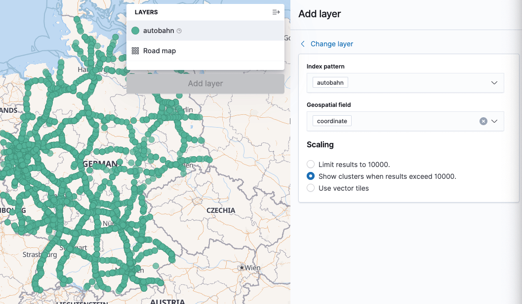
Make sure the autobahn index pattern is used (will be default, if there is only one) and the coordinate geo spatial field will also be selected, as this is the only geo_point field. Click on “Add Layer” - now it’s time for further customization:

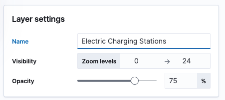
First, the name can be something like Electric Charging Stations.

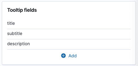
Second the tool tip fields should consist of the title, subtitle and description fields.

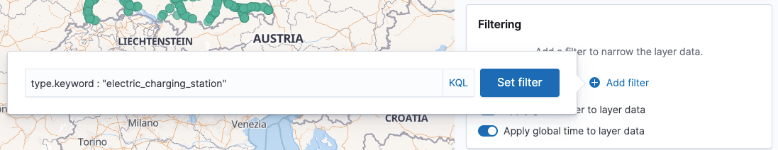
Third, we need to add a filter, for type.keyword : "electric_charging_station".

Fourth, let’s create nice icons via a icon layer style. There is a charging-station icon, I chose red as a color and set the border width to 0.

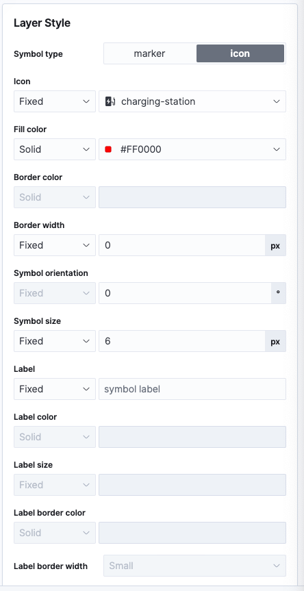
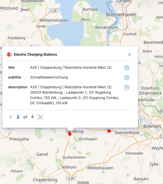
Click on Save & Close. This will leave us with a map like this plus nice tool tips. Back to our initial example from the A29, the tool tip looks like this:

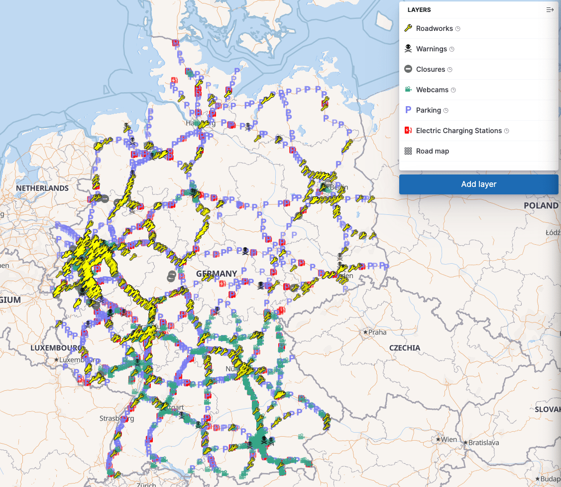
You can now repeat this process for all the different types and will end up with layers like this. My final result looks like this

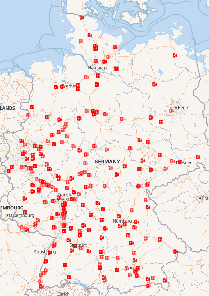
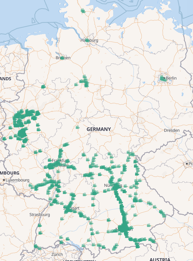
Now let’s explore this a little. Just checking the electric charging stations it seems, that there are much less in the eastern parts of Germany, probably due to the fact, that there are also less highways.

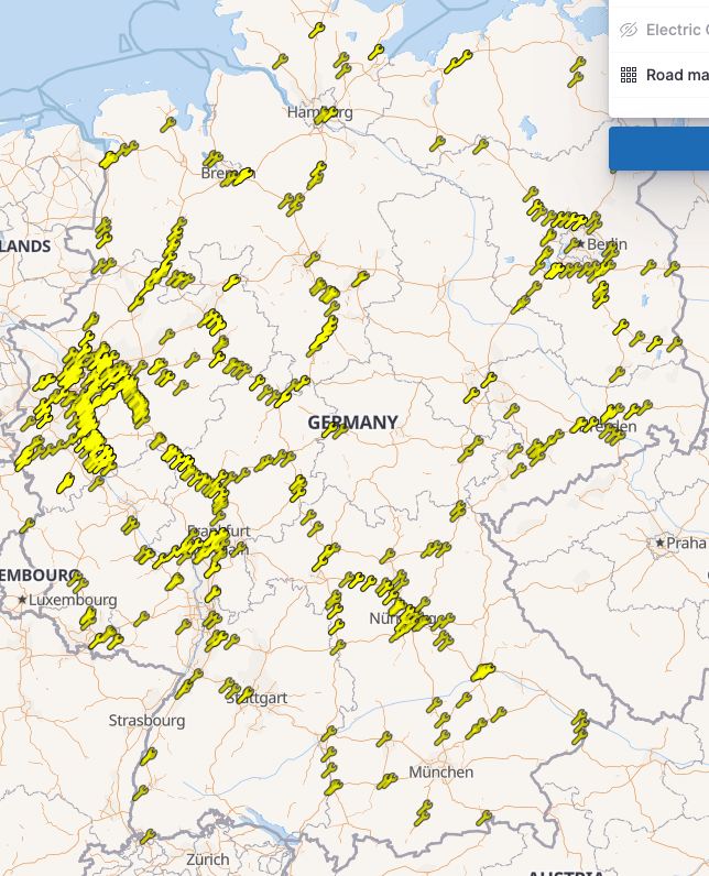
Showing the webcams only, there is a crazy density in Bavaria and southern Germany in general as well as in the Ruhr area, which makes sense as it is dense and very traffic jam plagued.

The roadworks layer looks like a density reflection of the most used highways across Germany.

So most of the data we looked at, was not real time, mainly because construction sites are usually staying for quite some time, even though there are some, that are only overnight. However, with warnings, things are a little different. My initial import only contained 57 warnings, let’s take a look at one:

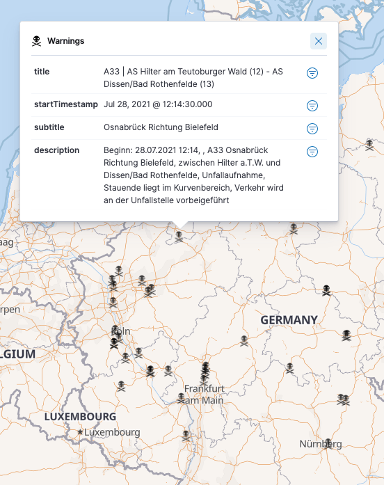
So this one happened about two hours before I started creating the maps layer, as I added the startTimestamp on the field. It does not seem as if there is an end timestamp, so things are supposed to expire automagically I guess.

The good news is, that due to the help of the @timestamp or the startTimestamp field, we could filter out warnings that are older than 24h and are not returned by the API anymore. All we need to do is to just rerun the above script.

Exporting the dashboard for sharing

You can now go ahead and save the visualization and also create a new dashboard at the same time. The advantage of creating a dashboard is, that you can easily export the dashboard and share it with others. Kibana has a dedicated Export Dashboard API that you can use to retrieve your dashboard and a Import Dashboard API to import a dashboard. Note: This is a Kibana and not an Elasticsearch API!

Summary

I hope you got a glimpse of how easy it is to get up and running with Kibana Maps, as soon as you ensure that your incoming data is in the right format to be able to index a geo_point into Elasticsearch. From then on, it’s all about adding the right layers in Kibana.

Last but not least, creating the data is one part, but make it easy for others to share, export and import dashboards as well.

If you want to rebuild this yourself, check out my gist with all the code required to run it.

Happy Mapping!

Resources

• Gist with the code
• Autobahn API GitHub Repo
• Autobahn App API OpenAPI
• bund.dev - more links to APIs ready for consumption
• GeoJSON RFC

Final remarks

If you made it down here, wooow! Thanks for sticking with me. You can follow or ping me on twitter, GitHub or reach me via Email (just to tell me, you read this whole thing :-).

If there is anything to correct, drop me a note, and I am happy to do so and append to this post!

Same applies for questions. If you have question, go ahead and ask!

If you want me to speak about this, drop me an email!

Back to posts