 Alexander Reelsen
Implementing search feedback loops - part 1
TLDR; This is a multi post series about implementing feedback loops in search applications that I had sitting in my drafts for quite some time. Instead of going high tech with the latest models, we try to make it as simple as possible and integrate this in our search queries.
Think of an e-commerce context with the examples provided in this and the following posts. This is where I am coming from. So everything here revolves around e-commerce product search.
Also note, that everything I show here is heavily simplified, the real e-commerce world and its product data is a wild beast to say the least.
What is a search feedback loop?
The idea of a feedback loop is to take user interactions into account when running a search, for example:
- Often clicked products are ranked higher
- Often bought products are ranked higher than clicked products
- Which products were found using the same search term that was typed in?
- Which categories did a search term belong to? For example a search for
iphone 17should probably rate products in thephonescategory higher than in thephone accessoriescategory.
One of the biggest drawbacks of such loops is reinforcement. If a product is displayed among the top 10 most of the time, it will also be clicked more often - disallowing other products that probably are great matches for a regular full text search to even occur in the top 10. The long tail products never get a chance.
Goal: Keep search understandable
The goal of this blog post series is to keep search understandable and try to integrate as much as possible into a search request, instead of having a complex chain of data science models to query before the request hits your search engine. The same applies for re-ranking. Also, often models are language specific - which in practice means, English is well supported, and then quality usually declines sharply. While again this is limited and such models might be more powerful, it will allow for a search request to be easily followed and make it explainable. Using your own data for searches also allows you to focus in your niche and the behavior of your users.
Setup
For completeness, here is my docker setup:
services:
  elasticsearch:
    image: docker.elastic.co/elasticsearch/elasticsearch:9.4.1
    container_name: elasticsearch
    environment:
      - discovery.type=single-node
      - xpack.security.enabled=false
      - ES_JAVA_OPTS=-Xms1g -Xmx1g
      - http.cors.enabled=true
      - http.cors.allow-origin=/https?:\/\/(localhost|127\.0\.0\.1)(:[0-9]+)?/
      - http.cors.allow-methods=OPTIONS,HEAD,GET,POST
    mem_limit: 2g
    ports:
      - "9200:9200"
    volumes:
      - ./data:/usr/share/elasticsearch/data
    networks:
      - elastic

  kibana:
    image: docker.elastic.co/kibana/kibana:9.4.1
    container_name: kibana
    environment:
      - ELASTICSEARCH_HOSTS=http://elasticsearch:9200
    ports:
      - "5601:5601"
    depends_on:
      - elasticsearch
    networks:
      - elastic

  web:
    image: python:3-alpine
    container_name: web
    working_dir: /web
    command: python3 -m http.server 8000
    ports:
      - "8000:8000"
    volumes:
      - ./web:/web
    networks:
      - elastic

networks:
  elastic:
    driver: bridge
This starts Elasticsearch, Kibana and a static HTTP server. Using the static HTTP server and ignoring all security rules we can directly query Elasticsearch from the browser - that’s why the CORS settings are required as well.
Using the python web server we can now build a sandbox, that directly queries Elasticsearch.
Requirement: A query sandbox
So what is a query sandbox? Essentially, whenever you want to play around with a query from your dataset, you need to compare current and new queries with your live data.
Especially within a company context such a sandbox fulfills several use-cases:
- Allow search engineers to test current queries with current data
- Allow product managers/engineering managers to understand queries and to test
- Share new queries among stake holders
- Easily modify existing queries
- Easily understand scoring (share the
explainoutput of Elasticsearch) - Advanced: Integrate with analytics data, to use the top 100 most common queries and compare their outputs
- Advanced: NDCG/MRR comparison
A sandbox is a good candidate to vibe code a PoC. Some sort of a split screen, that allows to load the existing query for a search term, a JSON editor and a result view to compare the results.
See this example screenshot:
Sample data
I also generated some sample data, around phone and phone accessories, but only 1k products. They look like this:
{
  "name": "iPhone 14 Pro 128GB Space Black",
  "base_model": "iPhone 14 Pro",
  "brand": "Apple",
  "category": "phone",
  "year": 2022,
  "year_feature": 3,
  "color": "Space Black",
  "weight_g": 206,
  "memory_gb": 128,
  "display_inch": 6.1,
  "megapixel_front": 12,
  "megapixel_back": 48,
  "battery_mah": 3200,
  "image_url": "https://placehold.co/300x300/3c3c3d/ffffff?text=iPhone+14+Pro+128GB+Space+Black&font=Roboto"
}
They represent names and some phone specific attributes. Note: if you had a much bigger and diverse catalog, attribute mapping would need to become a lot smarter, but let’s keep it simple for this example.
Mapping
{
  "products": {
    "mappings": {
      "properties": {
        "base_model": {
          "type": "keyword",
          "fields": {
            "text": { "type": "text" }
          }
        },
        "battery_mah":  { "type": "integer" },
        "brand":        { "type": "keyword" },
        "category":     { "type": "keyword" },
        "color":        { "type": "keyword" },
        "display_inch": { "type": "float" },
        "image_url":    { "type": "keyword", "index": false },
        "megapixel_back": { "type": "float" },
        "megapixel_front": { "type": "float" },
        "memory_gb":    { "type": "integer" },
        "name": {
          "type": "text",
          "fields": {
            "keyword":  { "type": "keyword" },
            "no_norms": { "type": "text", "norms": false }
          }
        },
        "weight_g":     { "type": "integer" },
        "year":         { "type": "integer" },
        "year_feature": { "type": "rank_feature" }
      }
    }
  }
}
The mapping allows for simple search, disables norms on one text field, and also has a rank_feature field, which we will see later. Let’s go through some sample queries of how one might tweak an initial query before going deeper.
Sample queries
Let’s start with the most simple search:
{
  "query": {
    "match": {
      "name": {
        "query": "<user typed query>",
        "minimum_should_match": "67%"
      }
    }
  }
}
This is probably the most simple query. Running against the name field,
and at least 67% of the terms need to match, so it takes the number of terms of the
input query into account. By not needing to match all the terms we can allow
for some tolerance towards typos, or misspellings (maybe even in our own
product data) or a user typing in a way too long search string (hello dear
agents).
By default, the length of the stored field is taken into account, but in
e-commerce you do not really care about the difference between
iphone 14 pro max and iphone 14 pro max 128 gb black in a product name,
so this could be taken out of the equation by disabling
norms
and then query accordingly (see the mapping above):
{
  "query": {
    "match": {
      "name.no_norms": {
        "query": "<user typed query>",
        "minimum_should_match": "67%"
      }
    }
  }
}
We can also query several fields like this:
{
  "query": {
    "multi_match": {
      "query": "<user typed query>",
      "fields": ["name^2", "base_model.text", "brand"],
      "minimum_should_match": "67%"
    }
  }
}
This query searches in name field with a boost, but also the base_model
and the brand field. This is a classic example, where you would need to
think about term-centric vs. field centric queries.
We could also take the age of a product into account, or the year it was released:
{
  "query": {
    "bool": {
      "must": [
        { "match": { "name": { "query": "<user typed query>", "minimum_should_match": "67%" } } }
      ],
      "should": [
        { "rank_feature": { "field": "year_feature", "saturation": { "pivot": 3 } } }
      ]
    }
  }
}
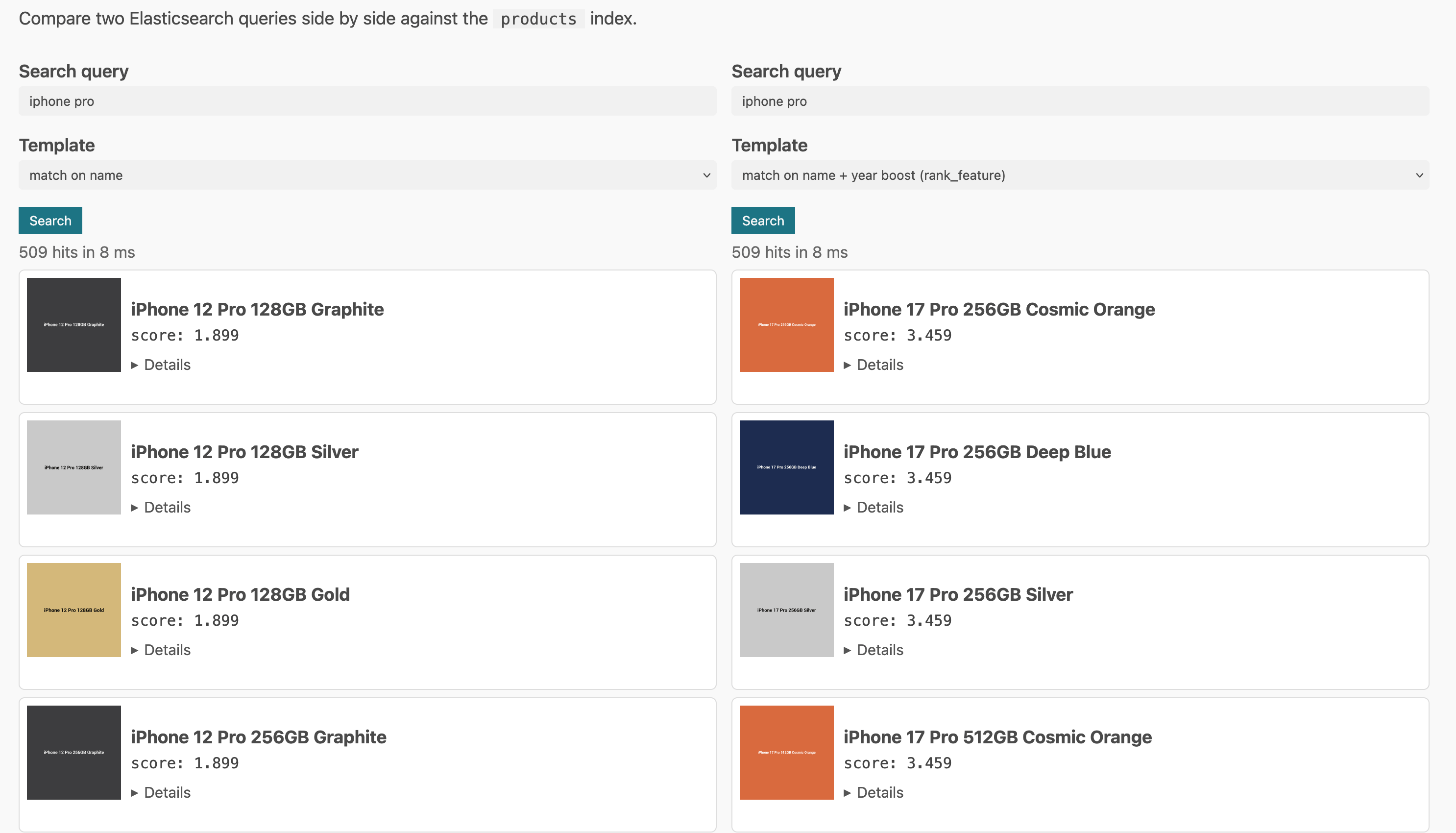
This will score more recent products higher, which often is what you want in an e-commerce setup - but not always :-)
Another common problem in e-commerce: Some terms are more important than
others, for example iphone 14 128gb yellow - probably the iphone 14 is
more important than the specs, because this is the model.
We could go with many variations here, like trying to be smarter about the number of words matched (or store shingles and search for terms right next to each other). We will skip this topic a bit to build some infrastructure to take clicks into account, so no need to focus on full text search only.
All of these queries have one issue. They only act on the input data of the products and never on any interaction with them. So if your product data is mediocre (or even worse, someone uses it to game your search engine, if you have smart sellers) you might have good results from a full text search perspective, but they will always be static. Let’s change that.
Taking clicks into account
In order to be able to take clicks into account, we first need some click data. A single record would consist of a timestamp and the product id in its most simple form. Before thinking about product data, let’s think about how we want the score to evolve over time. For this we need to take a look at different use-cases:
Constant popular product

This is your cash cow, and rarely happens that a product is constantly clicking well. Usually this means, it has been placed either in ads or has direct links from the main page or other well performing landing pages. This is a good reminder that clicks alone might not be a good metric, unless correlated with sales (or paid clicks are excluded). Maybe batteries are a good use-case for such a product, as they are in constant need.
This product should outscore all others in terms of a click score.
Constant semi-popular product

Not a high flyer, but something that probably gives you a solid revenue, so you should make sure, you have a few of those. Replacement parts or additional parts like specific charging cables might go into this category.
This product should also have a solid click score because of its consistency.
Recently hyped product

Classic flagship product use case, or a flagship product release, where the previously expensive product line got a lot cheaper and now finds a fair share of buyers. Phones are probably a good candidate here.
This is the first indicator that recency should be taken into account when creating a click score.
Past hyped product

Either something like a recently hyped product after a year, or a true short
term hype/one hit wonder triggered by some viral TikTok trend, or a seasonal
thing (pumpkin spice latte, however in this case this is not possible
because it would repeat after a year). Germans might remember the dubai chocolate
trend.
Recency here is even more important, as such a product is probably the least important of all the ones listed here.
Declining popularity product

Similar to the recently hyped product, but declining over a way longer duration.
Worth a discussion, if this or the constant semi popular product should have a higher click score (probably this one).
As you can see, recency definitely has to be taken into account into our formula, we cannot just take the average or total number of clicks per day or week and consider that a great formula.
As mentioned previously, in a real world example, you would also try to catch cheating by comparing with sales data, but again we will keep it simple here.
Also, there are dozens of other curves in real product data (when a campaign started etc), but again, we’ll keep it simple here.
Creating a recency based formula
OK, so what capabilities would our formula need?
- A single day should not be able to dominate
- Recency should be important (last months data is more important than last year’s)
- Volume: The more clicks a product has, it should get a higher score
- No need for incremental updates, full recompute is fine - this would change with a massive catalog (not a lot of e-commerce companies probably have such)
- The gap between popular and insanely popular should be relatively small, we’re more interested in diversifying products.
The input data looks like this for the product-clicks index and represents
a single event:
{
  "@timestamp": "2026-06-04T10:00:48Z",
  "product_id": "iphone-16-512gb-black"
}
For each product id, we need our recency based formula to be applied.
ESQL to the rescue
Instead of coming up with a complex scripted metric aggregation, ES|QL is of great help here.
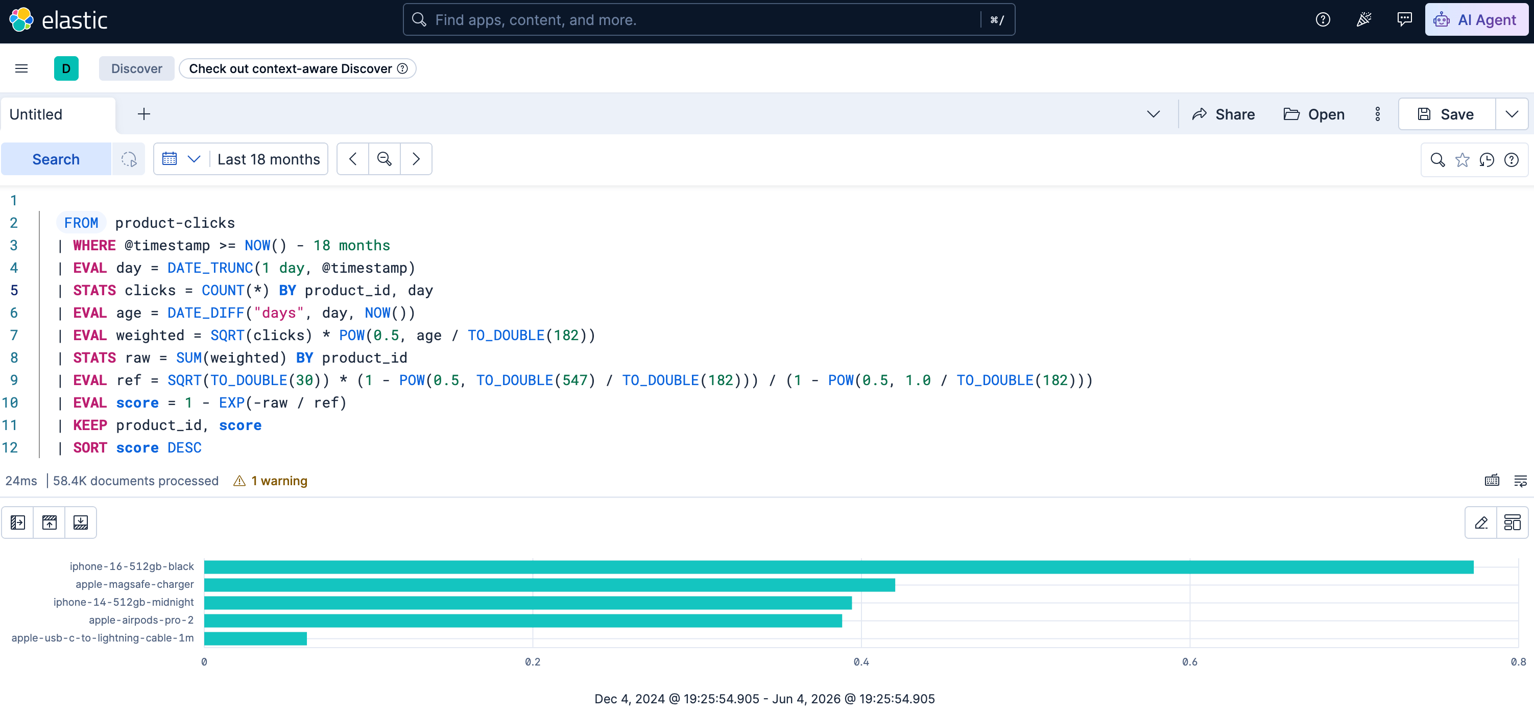
FROM product-clicks
  | WHERE @timestamp >= NOW() - 18 months
  | EVAL day = DATE_TRUNC(1 day, @timestamp)
  | STATS clicks = COUNT(*) BY product_id, day
  | EVAL age = DATE_DIFF("days", day, NOW())
  | EVAL weighted = SQRT(clicks) * POW(0.5, age / TO_DOUBLE(182))
  | STATS raw = SUM(weighted) BY product_id
  | EVAL ref = SQRT(TO_DOUBLE(30)) * (1 - POW(0.5, TO_DOUBLE(547) / TO_DOUBLE(182))) / (1 - POW(0.5, 1.0 / TO_DOUBLE(182)))
  | EVAL score = 1 - EXP(-raw / ref)
  | KEEP product_id, score
  | SORT score DESC
So, this is what this looks like in Kibana
Let’s dissect this query step by step
FROM product-clicks
  | WHERE @timestamp >= NOW() - 18 months
  | EVAL day = DATE_TRUNC(1 day, @timestamp)
  | STATS clicks = COUNT(*) BY product_id, day
This is grouping the data by product_id and day and counting the clicks.
  | EVAL age = DATE_DIFF("days", day, NOW())
  | EVAL weighted = SQRT(clicks) * POW(0.5, age / TO_DOUBLE(182))
This adds two new fields. age is the difference from the bucketed day till
now, weighted takes the square root of the counted clicks per day and
multiplies it by 0.5 to the power of age divided by the number of days of
half a year. So this value is higher the nearer the date is to the current
date.
| age | POW(0.5, age / TO_DOUBLE(182)) |
|---|---|
| 0 | 1 |
| 1 | 0.996 |
| 10 | 0.963 |
| 50 | 0.827 |
| 100 | 0.683 |
| 200 | 0.467 |
| 365 | 0.249 |
| 547 | 0.125 |
As this value is multiplied with SQRT(clicks) you will end up with higher
values when either the day is more recent or the number of clicks is high.
The next line
| STATS raw = SUM(weighted) BY product_id
is simply adding all the daily sums for each product id.
Now the next row looks static, but mainly because I used a script to create
the whole ESQL query with three constants in-lined. The 182 is essentially
the half-life, where we want the score to half (see the table above). 547
is roughly 18 months and 30 is the popular daily click rate, where we
consider a product to be popular - this could be calculated more dynamically
as your traffic patterns probably change over time.
| EVAL ref = SQRT(TO_DOUBLE(30)) * (1 - POW(0.5, TO_DOUBLE(547) / TO_DOUBLE(182))) / (1 - POW(0.5, 1.0 / TO_DOUBLE(182)))
Now the final task is score normalizing
  | EVAL score = 1 - EXP(-raw / ref)
  | KEEP product_id, score
  | SORT score DESC
How does it work? The basic idea is the expression 1 - e^(-x) is
normalizing all positive values into a value between 0 and 1. With
-raw/ref the sum of all clicks is used in combination with the formula
above.
Now with the output of this query, we can take the score for each product id
and index it into our products index, for example into a click_score and
click_score_feature field, so that we have these fields as rank_feature
and regular field (if you want to play around with it as part of a
function_score query). Also note, that rank_feature fields cannot
contain 0, so it must be a positive value.
A look at our use-cases
This example shows five products, which have the aforementioned characteristics and also show their score:
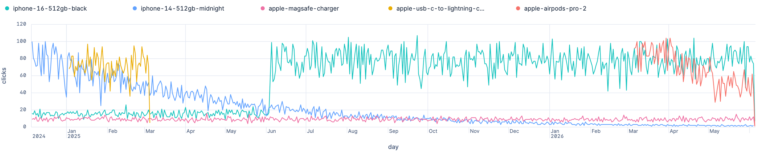
You can see the ids at the top, producing the following scores, applying the ESQL query from above:
iphone-16-512gb-black, score0.772, clicked a lot all the times, but has only been released within the time frameapple-magsafe-charger, score0.42, low traffic, but happening all the timeiphone-14-512gb-midnight, score0.393, clicked a lot at the beginning, but continuously fadingapple-airpods-pro-2, score0.388, short hype, relatively recent, slowly fadingapple-usb-c-to-lightning-cable-1m, score0.062, one hit wonder from the past, probably campaign driven
Integrating into the query
So how to integrate that into our query? We could go simple and use a
similar should clause, like previously
{
  "query": {
    "bool": {
      "must": [
        { "match": { "name.no_norms": { "query": "iphone 14", "minimum_should_match": "67%" } } }
      ],
      "should": [
        { "rank_feature": { "field": "click_score_feature", "linear": {} } }
      ]
    }
  }
}
Resulting in something like this
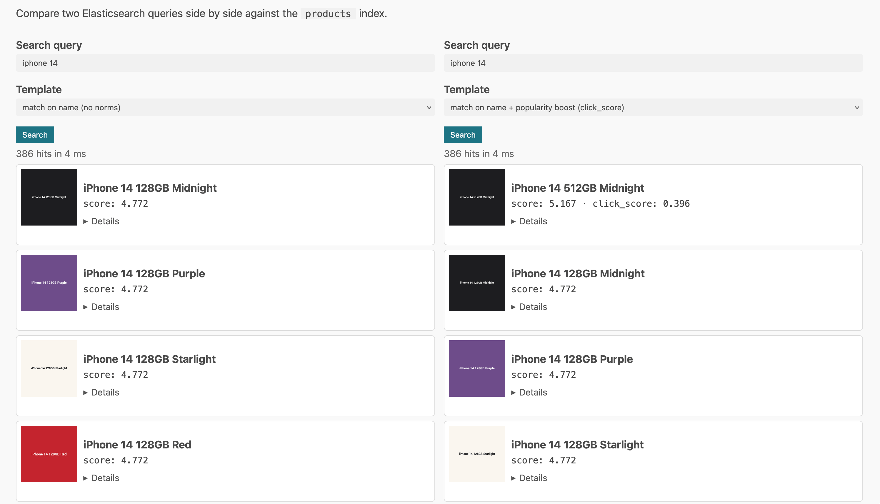
As you can see, the iPhone 14 with the click score is clearly scored above
the others. If you compare the scores, you could see, that the click_score
value of 0.396 was added to the full text score of 4.772. In many cases
you don’t know about the maximum value of the full text score, especially if
your boosting becomes more complex. You also do not know how much a value
of 0.396 will change the total score.
Normalizing full text scores
So, what can we do to normalize the score? Elasticsearch has a
function_score query that could be used for normalization. Within function
score you don’t have the max score, so you would need to do per document
score normalization doing something like this which is a bit lossy, as
high scoring documents end up roughly the same.
{
  "query": {
    "function_score": {
      "query": {
        "match": {
          "name.no_norms": { "query": "iphone", "minimum_should_match": "67%" }
        }
      },
      "boost_mode": "replace",
      "score_mode": "sum",
      "functions": [
        { "script_score": { "script": "_score / (_score + 1)" } },
        { "field_value_factor": { "field": "click_score", "factor": 0.1, "missing" : 0 } }
      ]
    }
  }
}
Also, this executes a script for every hit, which is not super performant.
Using the factor or k you could now influence the weight of the click
score.
Another alternative would be to go with a linear retriever depending on your license:
{
  "retriever": {
    "linear": {
      "rank_window_size": 100,
      "retrievers": [
        {
          "retriever": {
            "standard": {
              "query": {
                "match": {
                  "name": { "query": "iphone 14", "minimum_should_match": "67%" }
                }
              }
            }
          },
          "weight": 1,
          "normalizer": "l2_norm"
        },
        {
          "retriever": {
            "standard": {
              "query": {
                "bool": {
                  "should": [
                    { "rank_feature": { "field": "click_score_feature" } }
                  ],
                  "filter": {
                    "match": { "name": { "query": "iphone 14", "minimum_should_match": "67%" } }
                  }
                }
              }
            }
          },
          "weight": 0.1,
          "normalizer": "l2_norm"
        }
      ]
    }
  }
}
I wanted to test the minmax normalizer, but my dataset was too small so I
ended up with the same max scores, which normalized a lot of the data simply
down to 1 as the score, and then the ordering was relying on the click
score, which was not what I wanted (same applies with searching on fields
without normalization that creates a lot of similar scores).
I would probably go with the boolean query and the rank_feature in the
should part and play around with the different kinds of functions that are
supported (saturation, log, sigmoid and linear) as that seems to be the most
maintainable solution when looking at the query, albeit losing a bit of
control that you get with the retrievers.
Risks
Make sure you still have a search engine and not a ranking engine. If you
put too much weight into the click based score, newer products will have a
hard time coming up. Also multi year seasonality is ignored. You could add
another score for that and have one more should clause. Or have tags for
that like a field "tag": [ "black_week", "christmas", "carnival" ],
that gets a boost at a certain time of the year.
Summary
Reminder, this example mixed a square root of the daily clicks (to reduce
the impact of outliers), an exponential moving sum of these clicks using
time decay and saturation of that result. That’s the whole idea behind the
click_score.
Again, even though I begin to sound like a broken record, keep in mind that everything here is insanely simplified and should just give you some ideas, how to integrate a factor like clicks or sales into your searches without requiring to query a second system.
Usually you will not have the click data in Elasticsearch, but probably in your analytics system, like Google Analytics or something similar, so make sure it can be extracted. In order to make this easier to maintain, an algorithm that works incrementally would also help, so that there is no need to recalculate that number for every product and every day.
Whatever you change in your search, make sure you have the ability to A/B test built into your infrastructure.
Oh, and if you take anything from this article, it should be that you need some sort of sandbox mechanism with your data in order to help others understand your search.
Thanks for going through this article. I’m not yet sure what the next article will focus on, but we will again be using historical data to improve the present.
Final remarks
If you made it down here, wooow! Thanks for sticking with me. You can follow or contact me on Bluesky, Mastodon, GitHub, LinkedIn or reach me via Email (just to tell me you read this whole thing :-).
If there is anything to correct, drop me a note, and I am happy to fix and append a note to this post!
Same applies for questions. If you have a question, go ahead and ask!